Monday, October 7, 2013

A Collection of Interview Questions on Arrays


One dimensional array is probably the most important data types in programming languages. First of all, computer memory supports random access and can be treated as a big array. Second, other data structures can be implemented/simulated using arrays, e.g. strings, stacks, queues, binary heaps, linked lists, binary search trees, graphs can all be implemented using arrays. Because of this fundamentality, questions on arrays are commonly asked during a technical interview. The hardness level of such questions may vary from implementing a strcpy function to applying algorithmic tricks. In this post, I will try to cover a diverse set of these array questions, and I will keep this post updated when encountering new problems.

Coding interview questions usually test two aspects:

1. The ability to write correct and stylish programs. The interviewee should write syntactically correct C-family language code, and prove the correctness of the program by checking boundary conditions, loop invariants, etc. If the problem is relatively easy, not only the correctness but also the cleanness and readability of the code count.

2. The ability to think quickly and solve hard algorithmic problems. Google/Facebook/MSFT tend to ask tricky questions in their interviews. Most experienced programmers don’t think that using ACM/ICPC and algorithmic problems really test a programmer’s ability to code. However, this is a good way to see if the interviewee is clever or not (and clever people learn and adapt fast). More importantly, the coding of these problems will show how can you compact several coding tricks in, say, 20 lines of code.

Actually many problems here test both abilities, and in many cases writing correct programs with a good style weighted more than knowing the algorithmic trick to a specific problem.

Several problems in my collection are taken from a problem series by Chen Liren, link. If you read Chinese, I highly recommend this series, which contains many good questions and experience reports from real interviews.


The problem descriptions and some keywords use bold fonts.


Maximum subarray problem. This problem is so famous that it has its own Wikipedia page. It was popularized by Jon Bentley in his CACM column Programming Pearls and later collected in the book with the same name.

This problem can be solved in O(n) with O(1) space using dynamic programming. The DP solution itself is not very interesting. What interests me is two others solutions, one using a technique called cumulative sum, and the other using a more general technique -- divide and conquer.

Cumulative sum is a very useful pre-computing technique to allow O(1) range queries. It costs O(n^2) for the pre-computing thought.

Divide and conquer applies on a lot of sequence problems, including many sorting and searching algorithms. The trick is to design an O(n) merging step. In this problem O(n) merging is simple. In other problems, e.g. closest point pair, O(n) merging is non-trivial.

An extension of this problem is to find the maximum submatrix. An O(n^3) algorithm is expected.

Another variant of this problem: find two disjoints subarrays A and B such that |sum(A)-sum(B)| is maximized. Suppose A is on the left and B is on the right, for position i, we need the maximum/minimum subarray in range [1,i], and [i+1,n].

Given an array that is a rotation of a sorted array (elements are unique). The rotation of an array is to split the original array into two parts and concatenate the left part to the tail of the right part. E.g., {3,4,5,1,2} is a rotation of {1,2,3,4,5}. Now given this rotated array, find the smallest element.

Obviously we can do a linear scan and find the first number that is smaller than its left number. But linear scan costs O(n). Because the original array is sorted, it is natural to know binary search might get the running time to O(log n). In designing any binary search algorithm, it is important to prove that its correctness using loop invariant. [Bentley’s pearls and CLRS both cover loop invariant.] The algorithm sketch:

l=1, r=n

while a[l]>a[r] do
if (l+1==r) then
return r
m=(l+r)/2
if a[m]>a[l] then
l=m
else
r=m
return a[l]

Another binary search problem: given a sorted array, if A[i] == i, i is called magic index. Find the magic index.


Another binary search problem: given an array A=BC where B is a sorted array with non-increasing order, and C is a sorted array with non-decreasing order. Find B and C.


Not binary search, but incremental search: given an array A in which any two consecutive numbers diff by 1. Find the index of a target number T. E.g. A= {4,5,6,5,6,7,8,9,10,9}, and T=9.


Given an array of integers, write an algorithm that shuffles the array so that all odd numbers and ahead of even numbers.


This problem tests the understanding of quicksort algorithm. In quick sort’s partition procedure, once we fix a pivot, there is an O(n) algorithm that puts all elements less than or equal to the pivot to the left, and all elements that are greater to the right. In this problem, we shall redefine the comparison function that any odd number is “smaller” than any even number.


If C/C++ used, then write a general partition procedure which takes a comparison function pointer(C)/comparison operator(C++) as input would be nice.


A variant of this problem: 3-way partition. Given an array and i, design an in-place algorithm that puts all number < A[i] to the left, and all numbers = A[i] in the middle, and the rest in the right.


Another variant of partition algorithm: sort an array of 1/2/3 (don’t count # of 1,2,3), use a new partition algorithm instead.


Inversions. Given an array, calculates the numbers of pairs (i,j) such that A[i]>A[j].


This problem has several solutions. One is to modify the merge procedure in merge sort, to count the inversions in each merge procedure. Other solutions require using advanced data structures, and we don’t cover them here.

long long res; 

void merge(int l, int m, int r)
{
int n1=m-l+1, n2=r-m;
for (int i=0; i<n1; i++) L[i]=a[l+i];
L[n1] = INF;
for (int i=0; i<n2; i++) R[i]=a[m+i+1];
R[n2] = INF;

int j=0,k=0;
for (int i=l; i<=r; i++)
if (L[j]<=R[k]) a[i]=L[j++];
else { a[i]=R[k++]; res+=n1-j; }
}

void merge_sort(int l, int r)
{
if (l<r) {
int m=(l+r)/2;
merge_sort(l,m);
merge_sort(m+1,r);
merge(l,m,r);
}
}

Majority. Given an array of n integers, find the number that occurs more n/2 times, or report that such a number does not exist. E.g., in array {1,2,2,2,3}, 2 is such a number.


Solution 1: If such a number exists, then the n/2-th number in the sorted array must equal to it. Then we can first use a linear algorithm to find the n/2-th number in an unsorted array. In the literature, this k-th number problem is called selection problem, which has a complicated linear algorithm by Blum et. al. (four of the five authors of this paper were awarded Turing award!), and a O(n)-average time algorithm using quicksort variant.


Solution 2: a property of this problem: removing any two numbers that are different -> the frequent number remains the same. A walk through of the array using this property can get a candidate of the frequent number. Another linear scan checks whether the candidate occurs more than n/2 times.


A variant of this problem is to find a number that occurs more than n/3 times. The above two solutions still apply.


Given an array of integers, concatenate all numbers in some order so that the combined string is lexicological smallest. E.g., {3,32,321}, solution is 321323.


Define a new comparison operator of two numbers and sort the array. The new comparator is

compare x y 
if str(xy) > str(yx) then
1
else if str(xy) < str(yx) then
-1
else
0

The tricky part is to prove that this does yield the smallest string. To prove this order is correct, we need to prove three properties: reflexive, symmetric and transitive.


Given a sorted array and an integer x, output the number of times this integer occurs in the array.


Linear scan costs O(n). A straightforward binary search can spot the first occurrence of this integer, and we continue to count until the next number is not equal to it. However, this integer can occur O(n) times. A workaround is to do binary search again at the first occurrence. Suppose the first occurrence is at position i, and there are m numbers to the right. First, we check position i + m/2, if equal, we check i + m/2 + m/4, if not equal, we check i + m/4, and so on. However, this is non-trivial to get correct because there are a few boundary conditions.


The best solution to this problem is to use two binary search functions in C++ STL: lower_bound and upper_bound. lower_bound finds the smallest position i such that A[i]>=x, upper_bound finds the smallest position i such that A[i]>x. The solution to this problem is simply upper_bound(x)-lower_bound(x). The two functions already take care of boundary conditions and cases where x does not occur in the array.


Given an array of integers, all integers occur exactly twice except for one. Find the only integer that occurs once.


Use bit trick. x xor x = 0. (if a bit occurs twice, set it to 0)


Variant: Given an array, except for one X, all other numbers occur exactly 3 times. Find X.


Now bit trick does not work. However, the idea is the same. If a bit occurs 3 times, set it to 0.


Integers and sum. Subproblem 1: given a sorted array, find two numbers that sum to m. Subproblem 2: the array is not sorted. Subproblem 3: find four numbers that sum to m.


For subproblem 1, there is a trick called ruler reading. Keep two pointers to the left and right of the array, and move the pointers until the sum if m. O(n)


For subproblem 2, hasing or sorting.


For subproblem 3, there is trick called two-head search. First, we get the sums of all pairs (O(n^2)), sort these sums or put them in a hash table. for a+b+c+d=m, we now only need to enumerate a and b, and check whether c+d exists using binary search or hashing.


Another problem using ruler reading technique: given an array of positive integers, and S. Find a subarray with minimal length and the sum of the subarray is >= S.


Arrange 0 to n-1 in a circle, starting from 0, delete every m-th number. Output the delete numbers in sequence. E.g, {0,1,2,3}, m=2, the sequence is 1,3,2,0.


Solution: O(n), in every step, use module operation to find the exact number.


Given an array of integers, find a maximum subset that constitutes a sequence of consecutive integers. E.g., {15, 7, 12, 6, 14, 13, 9, 11}, the answer is {11,12,…,15}.


Obvious solution is to sort the numbers in O(n log n) and then do linear scan. The solution requires a running time better than O(n log n). Hint: make the consecutive numbers into same set, and use disjoint set algorithms to have O(n log log n) running time.


Given k sorted arrays, find a range [a,b] with minimal length such that each array has at least one element in [a,b].


Example,


1: 4, 10, 15, 24, 26


2: 0, 9, 12, 20


3: 5, 18, 22, 30


Minimal range is [20,24].


If we have all the numbers in k arrays sorted, and mark the numbers with labels 1 to k, then our minimal range should contain all k labels. This range checking can actually be done while we do merge sort of the k arrays. Hint: set a pointer for each array.


Given an array of 0/1, find the longest subarray such that the number of 0s and the number of 1s are the same.


Using the cumulative sum technique, the problem can be solved in O(n^2). Hint: fill 0 with -1, and use cumulative sum technique again.


Largest Rectangle in a Histogram. Given an array of heights, calculate the rectangle with largest area.


Solution: pre-compute two arrays L and R, L[i] indicates the most left position where h[L[i]]>=h[i].The following C++ code snippet calculates L (R would be similar):

int t = 0; 
for (int i=0; i<n; i++) {
while (t>0 && h[st[t-1]] >= h[i]) t--;
L[i] = t==0?0:(st[t-1]+1);
st[t++]=i;
}

Many other solutions to this problem: http://www.informatik.uni-ulm.de/acm/Locals/2003/html/judge.html


Variant: Given an matrix with 0/1, find the max submatrix with only 1s.


A much easier problem: given an unsorted array A, find in linear time, i and j (j>i), such that A[j] – A[i] is maximized.


In-place shuffle array: 1, 2, 3, …, 2n => 1, n+1, 2, n+2, etc. solution: Peiyush Jain, A Simple In-Place Algorithm for In-Shu?e. http://arxiv.org/pdf/0805.1598.pdf


Coins change problem. Given an array A and X, find how many subsets of A sum to X. Solution: DP.


Given two arrays S and T. Each is a permutation of 0 to n-1. By swapping 0 and another number repeatedly, change S to T. If minimal swaps are required, how to do it?


Solution: get a position correct in every step. If minimal swaps are required, use BFS/short path algorithm.


Given an unsorted array, find the longest arithmetic progression. Case 1: keep order of the original array. Case 2: no need to keep order.


Solution:


For case 1: use this hash data structure to store the n(n-1)/2 pairs of difference:


map<int, set<pair<int, int> >


difference -> sorted set of (i,j) pairs [difference = a[j]-a[i] ]


For case 2: since the order does not matter, we first sort the array in O(nlogn), and then the longest arithmetic progression is a sub sequence of the sorted array. This can be solved by DP:


dp[i][j] = dp[j][k] + 1, if i<j<k, a[i]-a[j]=a[j]-a[k]


dp[i][n-1] = 2, for all i < n-1


Given an array of n unique numbers from 1 to n, delete 1/2/k numbers, how to identify the deleted number/numbers?


For k=1, calculate sum.


For k=2, calculate sum and sum of squares.


For k=3, calculate sum, sum of squares, and sum of cubes.


Time: O(nk)


Another solutions: count the 0/1 bit at each position. Time: O(n log n)


An array of length n+1 is populated with integers in the range [1, n]. Find a duplicate integer (just one, not all) in linear time with O(1) space. The array is read-only and may not be modified. Variation: what if the array may be written into but must be left unmodified by the algorithm?


Solution: http://gurmeet.net/puzzles/duplicate-integer/ and


http://www.quora.com/Programming-Interviews/What-are-the-best-programming-interview-questions-youve-ever-asked-or-been-asked


The best solution requires solving several nontrivial subproblems, which are actually linked list problems!


Given an unsorted array A of n distinct natural numbers, find the first natural number that does not appear in the array.


I first saw this problem when reading R. Bird’s pearls of functional algorithm design, in which this problem is the first pearl. There are at least two good solutions (favor different tradeoffs) to this problem:


1. From 0 to n, there must be an integer that does not appear in A. We use an extra bool array with size n+1 and scan the array to mark occurred numbers. Then we can scan the bool array to find the first non-mark number as the solution. This solution is very easy to implement and costs O(n) time and O(n) space. Can we reduce the space cost?


2. Divide and conquer. Let’s check this property: from low to low+n, there must be a number that does not occur in A where low is the smallest (possible) number in A. We just need to guarantee that A does not have numbers smaller than low. Besides low, if we also know the upper bound value of A (we define upper bound as the number that is bigger than all numbers in A). So there are at most high-low distinct numbers in A. If and only if high-low==n, the numbers in [low, high) all occur in A once. If high-low>n, then there is a number in [low, high) that does not occur in A.


With this property, we can design a divide and conquer algorithm that in each step discard half of the numbers, the following is an implementation from Bird’s book:

minfree xs          = minfrom 0 (length xs, xs)
minfrom a (n, xs) | n == 0 = a
| m == b-a = minfrom b (n-m, vs) -- discard the numbers < b
| otherwise = minfrom a (m, us) -- discard the numbers >= b
where (us, vs) = partition (< b) xs -- partition in quicksort
b = a + 1 + n div 2
m = length us

This method uses O(n) time and O(log n) space. But the space cost can be reduced to O(1) if we write a iterative version of the above procedure. And different from linear selection algorithm which is only O(n) on average case, the algorithm here is strictly O(n).


Two problems on permutation arrays:


Find the next permutation. This function is implemented in C++ STL. Its Wikipedia page has a solution. The following is an OCaml implementation:

let next_permutation a = 
let swap i j =
let tmp = a.(i) in

a.(i) <- a.(j);
a.(j) <- tmp;
in
let n = Array.length a in
let k = ref 0 in
let i = ref (-1) in
begin
(* find largest i such that a(i) < a(i+1) *)
while !k<n-1 do
if a.(!k) < a.(!k + 1) then
i := !k;
k := !k + 1
done;
if !i = -1 then None (* if such i does not exist, no next permutation *)
else begin
(* find largest j such that a(j) > a(i) *)
let k = ref (!i + 1) in
let j = ref !k in
while !k<n do
if a.(!k)>a.(!i) then
j := !k;
k := !k + 1
done;
(* swap i j *)
swap !i !j;
(* reverse all after index i *)
let k1 = ref (!i + 1) in
let k2 = ref (n - 1) in
while !k1 < !k2 do
swap !k1 !k2;
k1 := !k1 + 1;
k2 := !k2 - 1;
done;
Some a;
end
end

Find the inverse of a permutation. E.g. A = [4,2,1,3] is a permutation, its inverse is B = [3,2,4,1], i.e. B[A[i]] = i (index starts from 1).


Solution: inverse several circle linked lists.


Problems with no good solutions yet:


Given an array A with length n, filled with 1 to n. Some numbers occur multiple times, some don’t occur. Identify these two groups of numbers in O(n) time and O(1) space.


Given an array, some numbers occur once, some twice, and only one X three time. Find X. (No solution yet)


Sunday, September 22, 2013

Kindle Wordbook -- Making a Personalized Dictionary from Books You’ve Read


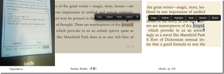
Kindle Paperwhite is really a good e-reader. Since I had it I have read and re-read several books with great joy and ease. As I am not a native English speaker, I rely on the dictionary function in Paperwhite. Of course, this dictionary looking function is implemented similarly in other software running on Android and iOS. However I found Paperwhite offers the best touch experience (In the appendix of the article, I compare the dictionary looking function in Paperwhite with iBooks and Duokan reader). Paperwhite is also more suitable for reading plain words than a tablet/phone, in terms of light, size, and battery life.

Kindle stores all the highlighted texts, bookmarks, and notes in a text file: My Clippings.txt. When I look one word in the dictionary, I will immediately highlight it. This highlighting action does not cost any extra touch because one touch is anyway needed to close the dictionary window.

my-clipping

Figure 1. My Clippings.txt opened in a text editor.

One problem with highlighted words is that they are just words -- they don’t carry the meanings in the dictionary, nor do they contain the context of the highlighted words. For many words that I have looked up before, when I later encounter them again, I still could not remember their meanings.

So my idea is to parse My Clippings.txt and find the highlighted words out and then

1) find the Chinese meanings of them using an online dictionary, and

2) find all occurrences in my past readings.

For the first task, I can use the API of an online dictionary. After some searching, I find www.wordreference.com provides a simple API. An alternative is dict.baidu.com, which can be accessed via HTTP requests.

If I just aim to get the Chinese meanings of the unknown words, then I only need to do the first task. However by merely looking at the Chinese translations of the words, I may easily forget some of them; and even I remember the vague meanings of these words, I still don’t know when and how to use these words. The vocabulary that we apply in writing and speaking is much less than that we can recognize while reading. By reviewing these words in their context, I can remember them better, and more importantly, by learning their usages in different texts by different authors, I can summarize when and how they are used. For example, I get to know the word `remorse’ while reading Mary Shelley’s Frankenstein and this word is then linked with various episodes and images in the novel. The word not only has a meaning, but has a more concrete feeling. Acquiring such a concrete feeling, I think, is a perquisite towards using the word confidently and correctly.

So I wrote a little Python program to do the two tasks automatically for me. The program can be downloaded at:

https://github.com/yinz/pwdict

And have a look at my recent words in browser:

image

Figure 2. View word book in a browser.

Python is very good at trying out ideas and making things done quickly because of its vast libraries and dynamic nature. In this project, I need HTTP requests, parsing json text, reading epub files, and parsing English sentences. There are libraries for all these tasks in Python. The HTTP and json libraries are built-in. And I modified epub2txt project to extract the pure text content from epub formats, which are typical book formats used across various mobile reading software. Parsing an article into individual sentences seems easy, but can be tricky in many special cases. So I used the NLTK library for this.

Appendix. Why dictionary looking in Paperwhite is better

Paperwhite: one touch to open dictionary, and one touch to back (marking the word does not cost extra touches)

Duokan and iBooks: two touches to open dictionary, and one touch to go back. Marking the word cost extra two touches!

dict-compare

Wednesday, July 17, 2013

Subtle Variable Scoping in R


A languages manual usually defines how a language behaves, but does not warn you in cases where you assume a feature should be supported but isn’t. As an example, I will talk about the subtle variable scoping in R language.

{} code blocks

A lot of programmers coming from C/C++/Java will assume that code blocks inside {} also introduce a new scope. However, in dynamic languages like R/Python/JavaScript/Matlab, code blocks do not introduce new scopes; only function does. This difference may cause some subtle bugs.

For example, the following R function returns a list of quadratic function objects:

make_funcs <- function(a, b, c_){
n <- length(a)
fs <- list()
for (i in 1:n) {
fs[[i]] <- function(x) {
cat(sprintf('eval %.1f*x^2+%.1f*x+%.1f where x = %.1f\n', a[i], b[i], c_[i], x))
a[i]*x*x + b[i]*x + c_[i]
}
}
cat(sprintf('variable i is still in the scope and has value %d\n', i))
fs
}


The input to this functions is three vectors of numbers which represent the three coefficients in quadratic forms. And let’s make three objects using the following coefficients:


a <- c(1,2,3)
b <- c(4,5,6)
c_ <- c(-1,-1,-1)


fs <- make_funcs(a, b, c_)

fs[[1]](1)
fs[[2]](1)
fs[[3]](1)


We are supposed to get three different function values. However, all the three functions are the same after checking the output:


> fs[[1]](1)
eval 3.0*x^2+6.0*x+-1.0 where x = 1.0
[1] 8
> fs[[2]](1)
eval 3.0*x^2+6.0*x+-1.0 where x = 1.0
[1] 8
> fs[[3]](1)
eval 3.0*x^2+6.0*x+-1.0 where x = 1.0
[1] 8


It seems that the three fs[i] use the same variable i when they are evaluated. That is, when the three functions are created, the R interpreter just remembers i as a variable in its parent function. Then the result can be explained: after the loop is finished, the variable i has value of 3, and it is still inside the scope of make_func.


Let’s see how will we write make_func in F#:


// a direct translation 
let make_funcs (a: int array, b:int array, c: int array) =
let n = Array.length a
let fs = new ResizeArray<(int -> int)>()
for i=0 to n-1 do
fs.Add(fun x -> a.[i]*x*x + b.[i]*x + c.[i])
fs.ToArray()


// a more functional translation
let make_funcs2 (a: int array, b:int array, c: int array) =
Array.zip3 a b c
|> Array.map (
fun (a0, b0, c0) ->
(fun x -> a0*x*x + b0*x + c0))


The following code would make three different functions as we expect:


let a = [| 1; 2; 3 |]
let b = [| 4; 5; 6 |]
let c = [| -1; -1; -1 |]

let fs = make_funcs (a, b, c)

fs.[0](1) // 4
fs.[1](1) // 6
fs.[2](1) // 8


Why F# code works as expected? When the three functions are created, they also know that variable i shall be found in the parent scope; however the three is have three independent scopes!


As the behavior in R’s version is definitely not what we want. How to make three different functions? Answer is make three different is in side a new function:


make_funcs2 <- function(a, b, c_){
n <- length(a)
fs <- list()
for (i in 1:n) {
fs[[i]] <-
(function() {
j <- i
function(x) {
cat(sprintf('eval %.1f*x^2+%.1f*x+%.1f where x = %.1f\n', a[j], b[j], c_[j], x))
a[j]*x*x + b[j]*x + c_[j]
}
}) ()
}
fs
}


Each time in the for loop, I create a new function and defines a variable j inside it, and the new function return the function(x). Notice that this new function is executed for n times in the for loop, therefore creates n different js.


This trick is ubiquitously used in JavaScript. For example instead of writing,


{
var a = 1;
//code blocks
}


we define a function and execute it immediately to make local variables:


(function() {
var a_is_hidden_from_outside = 1;
// in other words, no new variable in the global space is introduced.
}) ()


The assignment operators <- and <--


It seems that the block syntax {} can be translated as (function() {}) () in R/JavaScript. But in R, things can be more subtle. See the third version of make_funcs:


make_funcs3 <- function(a, b, c_){
n <- length(a)
fs <- list()
for (i in 1:n)
(function() {
j <- i
fs[[i]] <-
function(x) {
cat(sprintf('eval %.1f*x^2+%.1f*x+%.1f where x = %.1f\n', a[j], b[j], c_[j], x))
a[j]*x*x + b[j]*x + c_[j]
}
print(length(fs))
}) ()

fs
}

a <- c(1,2,3)
b <- c(4,5,6)
c_ <- c(-1,-1,-1)

fs <- make_funcs3(a, b, c_)

fs[[1]](1)


We translate {} after for loop as (function () {}) (), and now the assignment of fs[i] is inside the function wrapper. However, the code would not run correctly:


> fs <- make_funcs(a, b, c_)
ls length = 1
ls length = 2
ls length = 3

>
> fs[[1]](1)
Error in fs[[1]] : subscript out of bounds
> length(fs)
[1] 0


Obviously the variable fs is growing when the for loop is executed, however the variable fs inside the for loop is a different one from the one outside the for loop. And we find that the variable fs outside the for loop is only initialized but has not been added any new elements.


The assignment operator <- creates a new variables inside a function! It won’t search if the same variable name is in its parent environments! To do that which is what we suppose R to do, we have to use the <<- operator:


make_funcs3 <- function(a, b, c_){
n <- length(a)
fs <- list()
for (i in 1:n)
(function() {
j <- i
fs[[i]] <<-
function(x) {
cat(sprintf('eval %.1f*x^2+%.1f*x+%.1f where x = %.1f\n', a[j], b[j], c_[j], x))
a[j]*x*x + b[j]*x + c_[j]
}
cat(sprintf('ls length = %d\n', length(fs)))
}) ()
fs
}


And now this function should run as we expected.


Summary


In using R for interactive data analysis and plotting, most of time we won’t deal with these subtle language features. We just copy/paste some code snippet from R help and online and modify it to suit our own data analysis. However when we are into R programming, these issues do occur and will bite us when we assume our experience in C++/Java would also work in R.

Tuesday, July 9, 2013

Unicode Tips in Python 2 and R

Most of time, I don’t need to deal with different encodings at all. When possible, I use ASCII characters. And when there is a little processing in Chinese characters or other Unicode characters, I use .Net languages or JVM languages, in which every string is Unicode and of course when the characters are displayed they are displayed as characters (not as the unreadable escaped strings or Unicode IDs).

However recently I am working on projects on Chinese Weibo data, and I encountered some Unicode problems when using Python and R. (I use Python for data crawling and processing and R for modeling and visualization.)

This post is a note I start today and I will update it when I encounter new Unicode problems…

Python 2.7

Lesson 1: Normal string and Unicode string are two types. Do not mix use them.

When writing Unicode strings literals, we put a prefix u before the string:

>>> type(u'')
<type 'unicode'>
>>> type('')
<type 'str'>

Notice that the types of the two strings are different, one is 'unicode’, and the other is ‘str’. Python is a dynamic language and sometimes will do smart things between the two types. But we should use Python as if it is a strict static type language and never cross use the two types, and when needed, do conversions explicitly. See the following example: 
>>> u'abcd'.find('b')
1
>>> u'你儽'.find('儽')

Traceback (most recent call last):
File "", line 1, in
u'你儽'.find('儽')
UnicodeDecodeError: 'ascii' codec can't decode byte 0xba in position 0: ordinal not in range(128)


The first find operation works fine because it does not involve any non-ascii characters. The second won’t work because the two types don’t work with each other.


The error in the example seems simple to avoid. However when you load a set of text files from different sources, you may mix Unicode strings and normal strings.


Lesson 2: When passing a Unicode string to a function not written by you, check carefully whether that function supports Unicode.


It seems that if we have all the strings as Unicode strings in Python 2.7, we won’t have any problems. We can add u prefix to all non-ascii string in the file, and we also use codecs package to read Unicode files:


    with codecs.open(unicode_text_file, 'r', encoding='utf-8') as f:
read the file and all strings you get are of unicode type


Everything seems fine until we call function/packages that are written only for normal strings and we wished they would work for Unicode strings. For example, the csv package in Python 2.7 official release does not work with Unicode files. You cannot do things like:


    with codecs.open(file_profile, 'r', encoding='utf-8') as f:
reader = csv.reader(f)
head = reader.next()


The third line will throw UnicodeDecodeError just as above. So in Python 2.7 this is the pain point – you cannot expect all the common libraries that work nicely with normal strings to work nicely with Unicode strings. And a script that worked before for ascii files can suddenly fail on a Unicode file.


For library writers, it is pain too. Sometimes they need to write a special version for Unicode. I once worked with a human name parser in Python. European names can have accents on letters, but that library only accepts ascii strings. To use that name parser, I have to


1. Convert the name string into a normal Python string by removing all accents


2. Parse it using the library


3. Convert the result to Unicode string using .decode method


R


Lesson 1: In R, there is only one type of string, that is character. But this type can store whatever can be repressed as byte arrays. Think of R’s character type as C’s char[] and nothing more.


In Python, we have two types for two kinds of strings. In R, we have only one type for all kinds of strings.


My first problem is displaying Unicode characters in R. R’s default GUI and command line console cannot even display Chinese on a non-Chinese Windows. (On a Chinese Windows, you can only get a Chinese version R. Chinese characters are fine. However all info/error messages are also in Chinese, which are translated from English and which are just wired Chinese.)


When R is installed, it checks the System encoding. On Linux and Mac OS, the system encoding is usually UTF-8, and R uses that. However Windows is different, the following is my R session info:


> sessionInfo()
R version 2.15.1 (2012-06-22)
Platform: x86_64-pc-mingw32/x64 (64-bit)

locale:
[1] LC_COLLATE=English_United States.1252 LC_CTYPE=English_United States.1252
[3] LC_MONETARY=English_United States.1252 LC_NUMERIC=C
[5] LC_TIME=English_United States.1252


R’s default GUI then uses the encoding to display all strings. Of course, it fails on most Unicode characters.


Luckily the editor and the console in RStudio can display Chinese characters. And RStudio must have done some smart things:


> as.character(china_mapdata$NAME[1])
[1] "é»‘é¾™ę±Ÿēœ"
> "é»‘é¾™ę±Ÿēœ"
[1] "é»‘é¾™ę±Ÿēœ"
> as.character(china_mapdata$NAME[1]) == "é»‘é¾™ę±Ÿēœ"
[1] FALSE


The string in the data frame displays the same as the literal (the literal is represented as Unicode in RStudio console), yet they are not equal in many ways. This is because two strings display the same can be different in their internal representations:


> nchar("é»‘é¾™ę±Ÿēœ")
[1] 4
> nchar(as.character(china_mapdata$NAME[1]))
[1] 8


Their types are both character. However the representation are different: the literal is represented as 4 Unicode characters (4 chars * 3 bytes/char = 12 bytes) in the memory, and the string read from the data file is represented as 8 bytes (4 chars * 2 bytes/char = 8 bytes) in the memory:


> charToRaw("é»‘é¾™ę±Ÿēœ")
[1] e9 bb 91 e9 be 99 e6 b1 9f e7 9c 81
> charToRaw(as.character(china_mapdata$NAME[1]))
[1] ba da c1 fa bd ad ca a1


I find that the Chinese characters in the file I load the data frame uses GB2312 encoding. And because it is a binary file, I don’t have a simple way to change its encoding. But here is a method that I find:


# First write the data frame to disk
write.csv(china_mapdata, file = 'china_map.csv')
# In EmEditor, open it as GB2312, and SaveAs UTF-8
# Load the utf-8 file
china_mapdata <- read.csv('china_map.utf8.csv', encoding='UTF-8')
# Test
as.character(china_mapdata$NAME[1]) == "é»‘é¾™ę±Ÿēœ" # should be TRUE now


After converting all Chinese characters in Unicode, I can now follow the map example here (the author of the post, I believe, uses a Chinese Windows, therefore does not have my problem; All systems except Chinese Windows will encounter the coding problem though) :


ggplot(zhejiang, aes(x = long, y = lat, group = group,fill=NAME))+
geom_polygon(fill="beige" )+
geom_path(colour = "grey40")+
ggtitle("äø­åŽäŗŗę°‘å…±å’Œå›½ęµ™ę±Ÿēœ")+
geom_point(x=120.12,y=30.16,fill=FALSE)+
annotate("text",x=120.3,y=30,label="ę­å·žåø‚")


But when exporting the file as PDF, the Chinese characters cannot display correctly: 


image


After searching online, I find the solution in this SO question, and specifying the font explicitly solves the problem:


cairo_pdf("example.pdf", family="FangSong")
ggplot(zhejiang, aes(x = long, y = lat, group = group,fill=NAME))+
geom_polygon(fill="beige" )+
geom_path(colour = "grey40")+
ggtitle("äø­åŽäŗŗę°‘å…±å’Œå›½ęµ™ę±Ÿēœ")+
geom_point(x=120.12,y=30.16,fill=FALSE)+
annotate("text",x=120.3,y=30,label="ę­å·žåø‚")
dev.off()


The correct PDF output:


image


We can also change the font type to other Chinese fonts, refer their names here.


Some R’s functions can recognize the Unicode string, e.g. Encoding. I think such recognition is based on the first few bits of the string. But it does not recognize GB2312 string (Encoding function outputs ‘unknown’ for GB2312 strings). Magically RStudio in Windows (English version, locale set to Simplified Chinese) can recognize both strings and display them correctly.


Lesson 2: When dealing with Unicode in R, use a Chinese Windows (for Chinese only), or use Linux/Mac OS (which is by default UTF-8), otherwise you cannot display Unicode well.


See how Unicode code may be displayed in R's console (English Windows):


> head(zhejiang)
X.U.FEFF. AREA PERIMETER BOU2_4M_ BOU2_4M_ID ADCODE93 ADCODE99 NAME
223 222 9.277 26.825 224 33 330000 330000 <u +6D59><u +6C5F><u +7701>
224 223 0.000 0.103 225 1626 330000 330000 <u +6D59><u +6C5F><u +7701>
225 224 0.000 0.052 226 1634 330000 330000 <u +6D59><u +6C5F><u +7701>


The <u+xxx> symbols indicate that R knows that they are Unicode characters, however R cannot display them correctly. And these symbols occur as symbols in your plots as well, which is just meaningless. If R cannot display these characters as characters, how can we know what are they and how to use these characters in a plot?


To solve this problem, my solution is to use a Linux with UTF-8 encoding. This is the session info in my Linux virtual machine:


> sessionInfo()
R version 2.14.1 (2011-12-22)
Platform: i686-pc-linux-gnu (32-bit)

locale:
[1] LC_CTYPE=en_US.UTF-8 LC_NUMERIC=C LC_TIME=en_US.UTF-8 LC_COLLATE=en_US.UTF-8
[5] LC_MONETARY=en_US.UTF-8 LC_MESSAGES=en_US.UTF-8 LC_PAPER=C LC_NAME=C
[9] LC_ADDRESS=C LC_TELEPHONE=C LC_MEASUREMENT=en_US.UTF-8 LC_IDENTIFICATION=C


Summary


Conceptually Unicode in Python and R are quite simple. In Python, Unicode and normal strings have different types. In R, all the strings are represented as byte arrays (the good old C char[]!); so from its type, you cannot decide whether a string is Unicode or not. I think Python’s two-type design is good because the runtime exception will force the programmer to split normal strings and Unicode strings clearly (though it is headache, this is why Python 3 treat all strings as Unicode strings) .


What adds to the Unicode complexity is functions that manipulate Unicode strings and especially the display of Unicode characters on screens. A Unicode character is anyway 2-4 bytes in the memory, nothing special. When using Python and R for data analysis, we usually follow the REPL (Read–eval–print loop), it is meaningless to display Unicode as escaped strings. One cannot even judge whether the character is a Chinese character by reading the escaped strings! What’s worse is that different terminals may display differently for the same character. For example, in a Unicode-enabled Python console:


>>> print u'ä½ '
ä½ 
>>> u'ä½ '
u'\u4f60'


In a non-Unicode console:


>>> u'ä½ '
u'\xc4\xe3'
>>> print u'ä½ '
Äã
>>> print u'\u4f60'
ä½ 
>>> u'ä½ ' == u'\u4f60'
False
(In this example, the problem is not that the terminal cannot display Unicode characters, it is that the input characters in the terminal are not Unicode!)


The suggestion for the terminal and editor is


Use a Unicode terminal and a Unicode text editor when working with Python and R. For example, RStudio is, while Rgui.exe isn’t. PyDev plugin/PyScripter is, while the default IDLE isn’t.


And in Python, always put


# -*- coding: utf-8 -*-


at the beginning of the file, and save all source code files as Unicode.

Monday, January 28, 2013

A simple GUI tool to help find the right people


Today our professor asked us to find a list of researchers who are suitable as program committees for the big data conference:

2013 IEEE International Conference on Big Data (IEEE BigData 2013)

IEEE BigData is a brand new conference and does not have a “circle” yet. That means finding PCs is harder than other more established conferences. Our solution is to search the PCs in other major conferences such as WWW/KDD and find researchers who are doing big data.

After I count the number of PCs in SIGIR conference, I know that I need a tool to help me. SIGIR’11 has 223 researchers in its community! Think about repeating the following tasks for 223 times:

image

I want to automate the following the tasks:

image


There are two tasks that are hard:

1. Getting emails automatically. Some researchers simply don’t write emails on their webpages. To find the email, one have to open one of their research papers.

2. Decide if a researcher is related to big data. Actually we can formulate the problem into a binary classification task, which however requires some training data. So we go back to human labeling. Currently I define a set of keywords that indicate BigData:

let keywords =
    [ "large"
      "scale"
      "big"
      "data"
      "hadoop"
      "mapreduce"
      "distributed"
      "system"
      "cloud"
      "computing"
      "parallel"
    ]

and for each home page, I list the subset of keywords that occur in it. If no keyword is in his home page, then it is unlikely the researcher is doing something related to BigData. So the keyword filter is served as a helper for the human to decide.

I write an F# program and the code can be find on BitBucket. Here is a screen shot of running program:

image


When I click “WANT THIS”, the program inserts a record to the log file.

There two windows, one is for Google search and the other is for the page of the first search result. I keep two pages because occasionally the first result is not correct, I can then click other search results.

Some technical details:

1. WebBrowser in F# with only four lines!

let form = new Form(Visible=true, Text="Google Search Result")
let content = new WebBrowser()
content.Navigate("http://www.google.com")
form.Controls.Add(content)

2. Finding ralevtive path in an F# script (this makes the experiment easier to reproduce)

let folder = __SOURCE_DIRECTORY__ + @"\..\..\data\"

let logfile = folder + "log.csv"
let namelistfile = folder + "sigir10.txt"

3. Details in WebBrowser class

content.DocumentCompleted.Add(fun _ –> doing something when the page is fully loaded)

Tuesday, December 11, 2012

A reading list on F# and other ML languages


Yin Zhu

This page will be updated regularly.    last updated on 11 Dec 2012.


For F#, Don Syme has posted a blog page:

How to reference F# in a research paper?

Most of the papers therein are, of course, written by Don himself, the creator of F#.

The above page is on F#, particularly on the novel points in F#, e.g. active patterns, async IO, quotations, etc. But the most powerful part of F# is probably its ML heritage. To have a full and authoritative review of the core of F#, we must to back to the original papers of these ideas. This also motivated me to read some of these papers. For a few of them, I have quite a good understanding. However, as I haven’t had any formal training in programming languages (nor do I intend to – data mining is my primary job!), I only have a shallow understanding of most papers. So, I set up this page to keep track on interesting papers that I have read and want to re-read.

General ML

Paul Hudak. The conception, evolution, and application of functional programming languages. ACM Computing Surveys. 1989. pdf

A comprehensive survey. Tutorial on lambda calculus and its relationship to FP languages. Note the year it published, Haskell was not mature at that time.

Andrew Appel. A Critique of Standard ML. 1992. pdf

This paper gives a detailed review on ML language features, mostly from a user’s perspective. The concerns Appel raises are what a typical ML programmer would raise, e.g. the efficiency of the low-level implementation of datatypes.

David B. MacQueen. Reflections on Standard ML. 1993. pdf

This paper is another review on ML, but from a language designer’s perspective.

Module systems

Robert Harper and Benjamin C. Pierce. Design Considerations for ML-Style Module Systems. Chapter 8 in Advanced Topics in Types and Programming Languages. MIT. 2005. book link

An up-to-date review of the ML module system. It starts with a very general introduction, independent of any concrete implementations. At the end of it, it compares different of implementations (SML and OCaml), and compares the ML module system briefly to C and Java. This chapter does not build on the type book of Pierce and can be read alone.

David MacQueen. Modules  for  Standard  ML. 1984. link

Module extension to ML was primary designed by David MacQueen, and this paper is the first paper on ML modules. MacQueen wrote several subsequent papers on ML modules, e.g. implementation issues and separate compilation of SML modules.

Derek Dreyer. Understanding and Evolving the ML Module System. PhD thesis. 2005. pdf

To learn to use a concrete ML module system, the best way is probably to read tutorials and code. For OCaml, check Jason Hickey's introduction to Objective Caml, OCaml manual, many OCaml library designs(Map, Set, and particularly Jean-Christophe FilliĆ¢tre’s ocamlgraph).

Ad-hoc polymorphism

ML does not support typeclass/ad-hoc polymorphism. Attracted by the elegance of Haskell typeclass, many ML programmers want to use typeclass in ML. Without typeclass, ML programmers have to mimic a typeclass, e.g. dictionary passing is used for implementing F# powerpack’s matrix library.

Stefan Wehr and Manuel M. T. Chakravarty. ML Modules and Haskell Type Classes: A Constructive Comparison. 2008. pdf

It implements ML’s full module system using Haskell typeclass; and implement simple typeclass suing ML’s modules. Constructor typeclass is not implemented and everyone said it is hard or impossible (but I haven’t seen on the web why….)

Jeremy Yallop. Practical Generic Programming with OCaml. ML workshop’07. slides.

Another implementation of typeclass (again simple typelcass) using OCaml.

John Peterson and Mark P. Jones. Implementing Type Classes. PLDI’93. paper.

Philip Wadler and Stephen Blott. How to make ad-hoc polymorphism less ad hoc. POPL’88. paper.

The original paper of typeclass actually has suggested a simple implementation using explicit dictionary passing, and this technique as poor man’s ad-hoc polymorphism can be used in ML.

The realpower of Haskell comes from constructor typeclasses – Functor, Monads, etc, are all based on it. (I know how to use them in simple cases, however I have no idea how it is implemented and why it cannot be implemented in .Net; people keep saying that “to support higher-order typeclasses, the IL of .Net needs to be changed” however they never give any clue on why…)

Mark P. Jones. A system of constructor classes: overloading and implicit higher-order polymorphism. FPCA '93. paper.

Inside ML polymorphism

From a programmer’ view, ML polymorphism is quite easy to understand and use. However, normal programmers have little knowledge of the underlying theory and the implementation details of it. Also .Net and Java generics are heavily influenced by ML polymorphism (the core designers are from FP community). If one wants to know the generics in Java or .Net thoroughly, understanding ML polymorphism seems a good pre-course.

Robin Milner. A theory of type polymorphism in programming. Journal of Computer and System Sciences. 1978. pdf

This paper is the second most cited paper in ML literature (the first being the definition of Standard ML), the breakthrough in this paper, plus the ML module system, gives the modern shape of ML. The Hindley-Milner type inference scheme is also described in this paper.

Gilad Bracha, Martin Odersky, David Stoutamire and Philip Wadler. Making the future safe for the past: Adding Genericity to the Java Programming Language. OOPSLA'98.pdf

Andrew Kennedy and Don Syme. Design and Implementation of Generics for the .NET Common Language Runtime. PPLDI’01. pdf

These two papers are not directly related to ML. But since Java and .NET are the two major programming platforms today, understanding their implementations of generics is critical to programmers today.

Courses and tutorials

The following courses are taught by active researchers in this field. The instructors are not only good teachers of functional programming, but also successful researchers.

Cornell CS3110. Data Structures and Functional Programming. Uses OCaml. As the title says, data structures and OCaml are taught in an interleaving way. Well designed assignments. More theoretical stuff, e.g. fixpoints.

Harvard CS51. Introduction to Computer Science II: Abstraction and Design. Uses OCaml. Introductory course. Half OCaml and half Java. Focused on core programming abstractions, e.g. higher-order functions, modules, data types, lazy, objects, parallelism.

IT University of Copenhagen. Programs as data. Uses F# to implement a small compiler. Focuses on compilers implementation. At the end of the course, it also introduces Scala, and advanced abstractions, e.g. continuations and Monads.

Yale CS421. Compilers and Interpreters. Uses SML to teach compilers.

OCaml tutorials/books.

Tuesday, November 13, 2012

Reflection on Martin Odersky’s Scala Course at Coursera

Some F# news first:

Our team F# and Composite Networks, got the 4th place at the Stackoverflow Closed-Question prediction competition. And check out our beautiful visualization, “mapping the world’s programmers”, in which the location parser is written in F# and is open sourced. I will write more about this Stackoverflow project in future posts, but today is about Scala… 

--
Today I finished the last assignment of the Scala course at Coursera (code repository link removed due to course restriction). I must say this course is so well designed! As I am already familiar with F#, walking through the course is easy. There are a few things that are new to me or that I only had vague understanding previously. So after this course, I really feel that I have learned something and this is also why I’d like to write this reflection here, to share my fresh feeling of it.

Before this course, my only experience with Scala is an email judge program, which frequently scans an Email account and receive the new submissions from students and auto-score them. I used Scala because Java platform has a quite nice email library and has the example code for Gmail and also because I like to play new languages. The realtime scoreboard for that course is still online – it was really cool to watch this leaderboard when students made submissions. The source code is also in the repository. This program is written in one day (with copy&pate from a few snippets online). Scala is friendly to new users – as in day one I already become productive in it.

In the following, I will summarize the examples used in the course, unique language feature in Scala, homework  and a short language comparison to F# and C#.

1. Examples

The lectures, though mainly on simple materials, are well designed and well explained. Some of the classical examples are presented in the Scala language:

A. Newton’s method for calculating square root. Used as an example in higher order functions, stream/lazy evaluation. Later used to illustrate the concept of fix-point, but Odersky didn't go further to the fix-point in lambda calculus.

B. Rational number class. Numbers are the fundamental types in any programming languages. However usually they are built-in, and their implementations are hidden in the compilers or standard libraries. Implementing a Rational number is a great exercise in learning any language. From the number type, it can go as deep as class/object, comparison, type classes, passing operation dictionaries, etc.

C. Implementing functions as objects. The general idea is simple. What’s not simple is the variant. 

abstract class Function1[-S,+T] { 
  def apply(x: S): T 
}

There are rules and design patterns for when to use covariant/contravariant/non-variant. In Scala, the type checking for variant is much stronger than Java. This also adds complexity to the Scala type system and makes learning more involved. A complicated type system gives more power to library designers though. I will talk about this later.


D. Use List and binary search tree to implement IntSet. Scala does not have datatypes, so the implementation follows Scala's OO style.


E. Expression problem. This is a classical problem to discuss functional design and OO design. The best discussion I found was Ralf Lammel’s C9 lectures.


F. Fibonacci sequence and prime number sequence.


G. Classical search problem: n-queen for depth-first search (DFS) and pouring water for breath-first search (BFS).

Basically every example is implemented in several Scala ways, to show different language features of Scala, from simple to more advanced ones. For example, Fibonacci sequence first appeared in simple recursive functions and later in Streams as an example to show lazy evaluation/computing on demand.

The implementation for the examples is quite OO and trait is heavily used in all examples – actually you cannot avoid OO in Scala for everything concrete is an object.

2. Concepts

Besides the examples, I learn more about the following concepts:

A. Dynamic dispatching vs higher order functions. This is an exercise left at the end of one lecture. Odersky didn’t discuss it, but it is quite interesting to think about it. What I can think of is that .toString/.hashCode/.compare these universal methods associated with any object can be implemented as higher order functions.

Say in OO design, we have a Rational class that implements Order interface

class Rational implements Order { override int compare(other) { }}

In functional design, we would have (immutable) data and functions defined for them:

module Rational =
  type t = int * int
  let compare (a1, b1) (a2, b2) = a1*b2 – a2 * b2

When implementing a sort function, OO approach depends on dynamic method dispatch, while functional design uses higher order functions:

let sort (compare: Rational.t -> Rational.t -> int) (Rational.t list) = ...

The problem also reminds me of dictionary passing style for emulating type classes.


B. Subtyping vs generics, variant. (Lecture 4.4 & 4.5) I was confused about covariant and contravarint in C# and Java (there are major differences between the two). The variant problem becomes a problem when OO-style inheritance marries with FP-style generics. And definitely Scala has a very good solution in its language design. After the lecture and some more reading, I am clearer. But I think what I really need is to read through Scala’s standard library design to get more real-world examples and design lessons.

Variant + implicits are very powerful abstraction tools though the latter seems ad hoc.


C. By value, by name, and lazy. The lecture on Stream is amazingly clear, and it clearly differentiates three concepts: by value, by name and lazy.


D. for comprehensions are translated as map/filter/flatMap higher order functions. For compressions are easier to read than higher order functions. For example, Python, the language that keeps readability in its heart, encourages for comprehension over map/lambda syntax. This is particularly true when nested comprehensions are used, e.g. in the 8-queen example used in the lecture:

def queens(n: Int) = {
 def placeQueens(k: Int): Set[List[Int]] = {
   if (k == 0) Set(List()) 
   else
   for {
     queens <- placeQueens(k - 1)
     col <- 0 until n
     if isSafe(col, queens)
   } yield col :: queens
 }
 placeQueens(n)
}


3. Homework

The homework is well designed, which, as Ordersky reveals in an email to the email list, is from several TAs’ hard work. There are six projects; the skeleton of each project is already there, and each project has several holes to fill in. The primal exercise of doing these projects is thinking in types. Every function is fixed with a type signature, and the implementation I am asked to fill is usually one-liners. Placing the one-line-of-code that fits the type signature well is the primal problem in my head. After seeing six type-oriented design, I think when next time I need to design a project myself in Scala, it will come more naturally OO. (If you see my Scala email judge, you will immediately notice that I used Scala in an ML style…)

The other aspect of the homework is interesting. E.g. Representing a set as a function seems quite neat (though impractical because of efficiency), and using breadth-first-search for Bloxorz game is quite fun.

The hoemwork project also teaches test-driven development, for each project has a test suite, which is usually incomplete and requires the user to fill in more test cases.


4. Scala vs F#/C#


Qua work of art, the work of art cannot be interpreted; there is nothing to interpret; we can only criticize it according to standards, in comparison to other works of art. – T. S. Eliot, Hamlet and his problems, 1921.

This section is not about the course. But it is always interesting to compare languages, and in comparison, we learn.

My impression of Scala is that it is closer to C# than to any functional language. Scala is Java redesigned. The the core of Scala is OO. Then functional programming concepts and others are added based on its OO core. This is the same situation with C#. For language features, it seems to me that only Trait is unique in Scala, and Scala’s treat on variant is more sound. For other features, C# has them or can emulate them with little extra syntax. The fact that Scala is more complicate-designed than C# does not mean it is a better C#. I have seen discussions online arguing that Scala is too complicated and some early enthusiasts go back to Java after their projects become bigger and harder to manage.

On the functional side, Scala program can be very declarative, e.g. when using its immutable collections; however it is a another style of declarativeness which is different from ML family languages (F#/OCaml, and to some extend Haskell). In ML languages, the concept of function is everywhere – from simple function, to operators, to data constructors, functors, to even type constructors, it is a very consistent applicative style. While in Scala, from the very beginning, you think of an object, and then think about what can we do to this object.  This major difference becomes more evident when you actually begin to design a non-trivial project.


If Java platform has a soundly implemented ML, I would prefer that to Scala. However there is no ML there. If cross platform, concise and functional, performance of a statics language, a lot of libraries, etc, are kept in mind, then Scala seems to be a good choice among the very few. And recently the EPFL + Stanford joint team on parallel computing DSLs using Scala seems quite interesting and useful. There are also light-weight distributed frameworks written in Scala, e.g. Spark at Berkeley.


Summary


It is always entertaining to learn a new programming language, and I learned quite a lot by following this course. Thanks to Prof. Martin Ordersky and his TAs. It would be great if there will be a new and more advanced course next year. I would be interested in:

1. Design and implementation of the Scala collection library. Very few people write collection libraries, but many programmers need to design APIs for others to use. The Scala collection library is a gold mine to learn modern API design patterns.

2. Concurrent and parallel programming in Scala, using Actor, and other DSLs.

I will still use F# primarily for my data mining projects. And when I need a Java library or serious cross platform, I can rely on Scala.